
摘要: Using machine learning for anomaly detection has been all the rage in recent times but according to withering critique by Renjie Wu and Eamonn J. Keogh last year, it’s possible the gains have been illusory.
▲From Current “Time Series Anomaly Detection Benchmarks are Flawed and are Creating the Illusion of Progress” by Renjie Wu and Eamonn J. Keogh
Using machine learning for anomaly detection has been all the rage in recent times but according to withering critique by Renjie Wu and Eamonn J. Keogh last year, it’s possible the gains have been illusory. I’ve been working on a solution to anomaly detection, which I make more explicit here. But this post first outlines their critique of the status quo. You can read it in Current Time Series Anomaly Detection Benchmarks are Flawed and are Creating the Illusion of Progress (paper).
Triviality
I’ve always been instinctively wary of the term “anomaly” as it seems to invite circular definitions. (I kid you not that as I write this my dog is actually chasing its tail on the floor beside me). My mild skepticism is nothing set against the brutality of Wu and Keogh’s review. In writing about recent uses of variational auto-encoders for anomaly detection they write:
“much of the results of this complex approach can be duplicated with a single line of code and a few minutes of effort.”
Ouch. The authors use this “one line of code” yardstick to assess recent alleged advances in anomaly detection, leading to the identification of what they say is the first flaw in benchmarking. They define a time-series anomaly detection problem to be trivial if it can be solved by using a primitive function such as mean, max, std (as compared with a one-line call to kmeans or whatever).
The authors claim that the Numenta benchmark used in Unsupervised real-time anomaly detection for streaming data by Ahmad, Lavin, Purdy, and Agha (paper) is trivial in this sense. That’s also true of the NASA dataset used in Detecting Spacecraft Anomalies Using LSTMs and Nonparametric Dynamic Thresholding by Hundam, Constantinou, Laporte, Colwell, and Soderstrom (paper), they reason, because most of the anomalies diverge from the norm by orders of magnitude.
Some participants in the reddit discussion felt that the one-line criterion is unacceptably vague — but I personally don’t have an issue and I think they might be missing the larger point.
Unrealistic Anomaly Density
Wu and Keogh note that in some benchmark data sets, there are large contiguous regions all marked as anomalies; or many regions marked as anomalies; or anomalies very close to one another. They exhibit the following case from a Yahoo benchmark dataset and note that A is classified (manually, we presume) as anomalous whereas B is not.
This clearly creates a problem because there is no difference between A and B — nothing has changed and just about any reasonable algorithm would treat them the same (unless it had some arbitrary counting going on, perhaps).
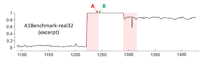
▲From Current “Time Series Anomaly Detection Benchmarks are Flawed and are Creating the Illusion of Progress” by Renjie Wu and Eamonn J. Keogh
Here’s another example from the Yahoo benchmark dataset. Can you tell which of the points C and/or D is considered to be anomalous, for the purpose of benchmarking algorithms? Yes, the red line gives it away. In the creation of the dataset, C is considered an outlier whereas D is not.
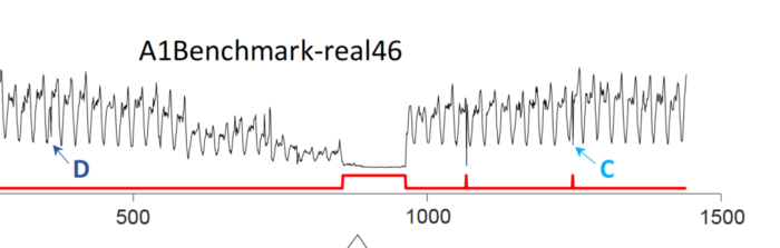
▲From Current “Time Series Anomaly Detection Benchmarks are Flawed and are Creating the Illusion of Progress” by Renjie Wu and Eamonn J. Keogh
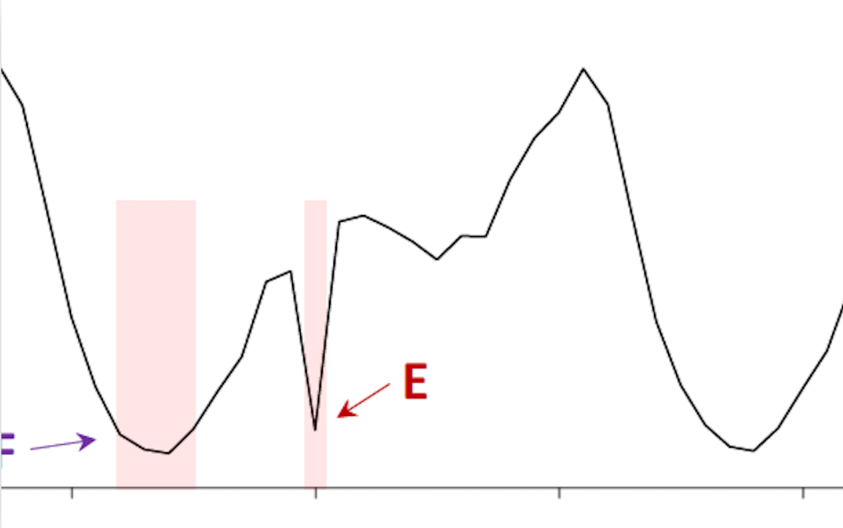
This brings us to the apparent circularity of the problem — one I shall propose a solution for in due course. However, first, let’s borrow yet another example from the keen eyes of Wu and Keogh.
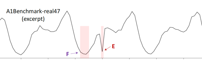
▲From Current “Time Series Anomaly Detection Benchmarks are Flawed and are Creating the Illusion of Progress” by Renjie Wu and Eamonn J. Keogh
Why is F an anomaly? Your guess is as good as mine, and unfortunately this kind of “ground truth” is being used to report progress in anomaly detection. I won’t go on, but see the paper for more examples of dubious choices.
Run-to-failure bias
The Yahoo benchmark, which as you infer takes quite a beating in Wu and Keogh’s paper, suffers from another flaw — the distribution of anomalies is highly skewed. This plot shows just how bad that bias is. The vast majority of data points considered to be anomalous are at the very end of the time-series. So an algorithm that takes this into account will outperform others — without, obviously, providing any genuine advantage in the wild.
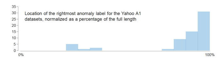
▲From Current “Time Series Anomaly Detection Benchmarks are Flawed and are Creating the Illusion of Progress” by Renjie Wu and Eamonn J. Keogh
Solution #1: Better benchmark datasets
The authors suggest that there are other issues with recent research as well, including questionable choices of scoring functions and unclear definitions of the domain of application. But I will refer the reader to their paper, as I would like to move this to a more positive note.
Having seen some of the difficulties in the datasets used for anomaly detection benchmarking, one obvious solution is the creation of better ones. The authors strongly suggest abandoning the existing benchmarks and they have created their own — adding to the growing collection of UCI’s datasets.
However, I for one am not sure that this really gets at the heart of the circularity of time-series anomaly detection. For instance, how would one characterize a jump in the price of bitcoin as anomalous or not? What does that really mean? What does it mean for an algorithm to be good at detecting, or classifying after the fact, anomalous behavior?
While Wu and Keogh suggest throwing out the anomaly detection datasets, I’m tempted to suggest that perhaps we should throw out the term anomaly until someone can provide a workable definition — because clearly, the field seems to be struggling in this regard. We already have the word classification (into “things Bob thinks are anomalous” or “things Bob thinks are within the normal operating range”) and if papers were titled “A novel machine learning approach to classifying things Bob thinks are anomalous” I’d say there’s less danger of anyone getting carried away, or confused.
Can this idea be followed to its logical conclusion? Let me introduce you to a competition-based notion of anomaly that isn’t circular or ambiguous.
Solution #2: Market probabilities and “Z-streams”
When I ask myself if a move in bitcoin is anomalous (which actually I don’t, because I hate the word) I simply look at the following plot. This, my friends, is a z-stream and as revealed in the underlying mechanics it could be construed as a generalization of the classification definition given above, except we replace Bob with Bob, Mary, and Alice and we ask them to “classify” data into percentiles.
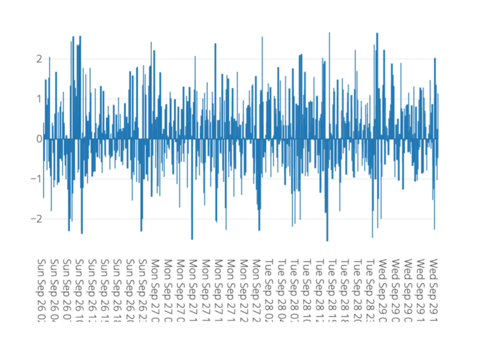
▲Image from www.microprediction.org
I would prefer you look at is the live version of this z-stream, by the way, because you can click on the Go To Parent button and reveal the time series of Bitcoin price changes here that, in combination with predictions made by algorithms shown on the leaderboard, determine the ‘z’ values.
To emphasize, these numbers aren’t the result of some fixed algorithm. Here’s how they are computed (the short version of this post).
- Algorithms submit 225 guesses of the future value of a stream of data, knowing they will be rewarded based on how many are close to the subsequently revealed truth.
- The sum of all submitted guesses is easily interpreted as a cumulative distribution F (for instance one could use the empirical distribution, but there are arguably better ways).
- An arriving data point x is assigned a z-score equal to z = norminv(F(x))
The claim is that z will be close to normally distributed because if not, there is an incentive for reward-seeking prediction algorithms to fix it.
(As an aside, there isn’t a strong reason to apply norminv, and we could talk in percentiles instead. However, there is some evidence that algorithms and their authors often prefer transformed time-series. See the paper by Tommaso and Helmut, for example.)
Bob, or the reader, can create another algorithm and launch it any time they want to — by modifying a Python script (like this one) and running it. Furthermore, Bob, Mary, and Alice shouldn’t have too tough a time adding better algorithms because Alice can rather easily draw on any of a hundred of so fully autonomous time-series point-forecasters ranked here.
Further lowering the cost of fixing the distribution, a dozen popular Python time-series packages are exposed in a canonical sequence-to-sequence calling signature here, hopefully making Alice’s life easier as she tries to make distributional predictions of Bitcoin price movements (for instance she can predict volatility). And Alice has some small monetary incentive to add her algorithm to the mix, though I’m sure that pales beside her scientific motivations.
Now I admit that the use of ‘z-score’ might be considered a confusing overloading of existing terminology. My intent was that the numbers in z-streams would be reminiscent of z-scores but at the same time, clearly superior. And my writer’s block aside, we are now free to define an anomaly in numerous ways using the z-curve time-series. More on that in a moment.
Anomaly horizons
But first, here’s yet another potential issue with anomaly detection research, and the creation of anomaly data sets. There often seems to be no notion of term-structure. Yet in the real world an event might be considered anomalous on a short time scale but not a longer one, or vice versa.
It is impossible not to confront this issue in engineering the z-streams. So you will notice that each z-stream is defined relative to a prediction horizon. Those horizons are currently just over one minute or just shy of one hour. When a new data point arrives, we look back to the submitted predictions and use only those that were received prior to a cutoff time.
I hope that is clear from the mechanics.
The only thing anyone will agree on
It’s an old idea to define probability as the outcome of probabilistic competition.
De Finetti famously declared that probability does not exist … unless people are betting on two flies crawling up a wall. That’s my Australian riff on the Italian mathematician’s ponderings in the 1920’s onward, anyway. Today we speak of risk-neutral and market-implied probability because finance stole the idea and renamed it.
The French invented the parimutuel for cock-fighting, which is a special case of the mechanism underlying the z-streams I have shown you. An English-born Australian inventor implemented the totalizator in 1907, but the New Zealanders were the first to use it in anger. There’s plenty of credit to go around.
In the domain of frequently repeated prediction, risk-neutral probability coincides more or less with actuarial probability (to try to use a word suggesting real-world probability without starting a fight between Bayesians and Frequentists). We have less to worry about.
And in that domain, which I refer to as the microprediction domain, the self-regulating nature of competitive prediction (for instance competitive distributional prediction) means that we avoid most of the usual problems with the assessment of time-series algorithms — such as data leakage and overfitting. We replace them with engineering headaches instead.
The main assumption here, and it will be tested over time, is whether small rewards are enough when the amortized frictional cost of participation is low (say for an itinerant algorithm foraging the network of streams — you can create your own “crawler” rather easily).
Notice also that the z-stream values fall out because the parent contest demands distributional predictions. And not only is there an incentive for Mary to put more mass where it is missing, but there is a second, mildly sneakier incentive provided by the lottery paradox (discussed here).
As I have previously noted, live, distributional, streaming contests also happen to be considered the future of forecasting assessment according to the experts who arrange M-Competitions, and have done so for forty years.
Engineering custom anomaly detection using z-streams
If you want z-stream values for existing streams (listed here) you have them. There are many options for that. However, chances are you’ll have your own bespoke data.
To create a new parent stream similar to the Bitcoin one, you can use an API or Python client library (“microprediction”) to publish your own data (see instructions).
That will automatically create a secondary contest stream where your z-values are predicted, by algorithms like this one. Then, you might want to go one step further and use the z-values to define some other customer number that you think reflects the operational needs.
The cycle repeats. What will best predict your own anomalies? I can’t say but here’s one idea. Changes in the relative performance of time-series algorithms might be a harbinger of anomalous behavior (as when an algorithm that specializes in predicting sequences of zeros charges up the leaderboard — though we can construct more nuanced examples obviously).
Now I hope it is clear how this might serve academic purposes as well as live business needs. And it should also be clear that triviality is no longer a bug. Maybe it is a feature. Now one-liners are actually meaningful, if applied to z-streams for instance.
I’m quiet, for now, on the matter of what functionals of z-streams are appropriate. I’d rather just provide you the raw materials. But one might define an anomaly as a sequence of z-curve points of length k, the absolute value of whose sum exceeds a threshold. Alternatively, it could be a run of z-curve values all above a threshold, or a run satisfying some other probabilistic metric.
The z-curve construction also engineers us away from run-to-failure bias, or other biases, which could unfairly advantage mercenary algorithms gaming the contest. The issues with silly densities of anomalies are now a non-issue too.
Perhaps there is something I’m missing, but if not, I will be interested to see if academic researchers make use of this device, or whether they continue to chase their tails instead.
轉貼自Source: medium
若喜歡本文,請關注我們的臉書 Please Like our Facebook Page: Big Data In Finance

留下你的回應
以訪客張貼回應