
摘要: The Gaussian Mixture model (GMM) will be used to detect different moods in the stock market. The GMM model will be applied twice: first using price data, and subsequently with macro-economical data.

▲Photo by Element5 Digital on Unsplash
Introduction
Over the last decade, the stock market has become increasingly accessible to the average layman. Moreover, the volume of money entering and exiting the market each day is at an all-time high.
As an investor, you can hone your acumen for when to buy or sell in many ways. A common approach is consulting friends or fellow investors, who quickly inundate you with conflicting opinions.
I will approach this golden, money-making question — when should I buy or sell? — with rigorous mathematical tools rather than blunt opinions. However, it is crucial to note that ultimately, people’s opinions and speculations drive the market; the mathematical tools will hopefully capture this mood or opinion.
I will demonstrate how the Gaussian Mixture Model can be used to help determine when money should enter or exit the market.
Mathematically, the mood of the market at any given time can be referred to as the “market state”. The mood can typically be interpreted as any number of concepts such as a bear or bull market; the degree of volatility; fire and ice, etc.. The way we name each state is far less important than clustering similar trading days together based on some shared characteristics.
Due to the fact that there is no clear definition for the mood of the market — and therefore, no response variable to represent the market — an unsupervised machine learning model is best to classify the market into states.
Supervised vs Unsupervised machine learning
The difference between the two approaches is the use of labeled datasets: supervised learning uses labeled input and output data, whereas an unsupervised learning algorithm does not. A labeled dataset is where the response variable, or the variable you are trying to predict, contains either numerical or categorical values. Hence, when you are using a supervised machine learning algorithm, the prediction variable is clearly defined. One very simple, but powerful, example of supervised learning is linear regression.
Gaussian Mixture Model (GMM)
The gaussian mixture model is the overlapping of multi-normal distributions in p-dimensional space. The dimension of the space is generated by the number of variables. For example, if we had one variable (S&P 500 returns), the GMM would be fit based one dimensional data. The GMM can be used to model the state of the stock market along with other financial applications. One characteristic from the stock market returns, is heavy tails, which are generated from days of high volatility. The ability to capture highly volatile days in the tails of the distribution is important for capturing information in the modelling process.
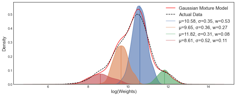
The above graph represents some multimodal data with 4 clusters. The Gaussian mixture model is a clustering type of model used to label data.
One main benefit of using the GMM for unsupervised clustering is the space encompassing each cluster can take on a ellipse shape. Gaussian mixture models take not only means into account but also co-variance to form a cluster
An advantage of the GMM approach is that it is entirely data-driven. The data given to the model will form the clusters. Importantly, the labelling of each cluster can be numerical, as the data drives the underlying characteristic, rather than human opinion. However, it can be hard to put intuition behind the resulting market conditions.
Mathematics of the GMM
The goal of the Gaussian Mixture Model is to assign data points to one of n multi-normal distributions. To do this, an Expectation Maximization (EM) algorithm is used to solve the parameters of each multi-normal distribution.
- Step 1: Randomly initialize the starting normal distribution parameters
- Step 2: Preform the E-step or the expectation step
- Step 3: Preform the M-step of the maximization step
- Step 4: Calculate the log likelihood of the joint probability of (Data given fraction of each state , mean , covariance)
- Step 5: Repeat steps 2–4 until the log-likelihood converges
The probability that each data point belongs to a certain cluster is given below. Based on the indexing, we are given a probability of each data point belonging to each induvial cluster. The size of the matrix will be the number of data points by number of clusters. Since it is a probability matrix, the values will sum to 1 under index ‘i.’
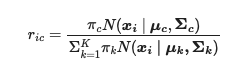
The interpretation is as follows: the index i represents each data point or vector. The index c represents that given cluster; if we were to have three clusters (c) would be 1 or 2 or 3.
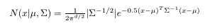
▲Multivariable Gaussian Formula
The multivariable Gaussian formula is given where mu and sigma are parameters that require estimating using the EM algorithm.
An additional key concept is that each gaussian distribution in our space is unbounded and overlapping with one another. Based on the location of the data point, a probability is assigned to it from each distribution. The probabilities for each data point belonging to any of the clusters will sum to 1.
Lastly, since the EM algorithm is an iterative process, we need to gauge the progress at each step to know when to stop. To do this, we use the log-likelihood function for the model to measure when our parameters are converging.

Implementation of the GMM
This section will be broken-down into two sections each representing an application of the GMM.
- Classification of the S&P500 returns into three states using a GMM
- Classification of the American economy using Macroeconomics data fit with a GMM
Section 1 : Classification of the S&P500 returns into three states using a GMM
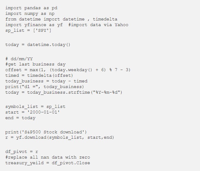
The first section will use daily return data from the S&P500. The data was received from yahoo finance.
Firstly I need to determine which factors to consider for detecting which market state we may be in. Secondly I need to determine how many states would best represent the market environment. Here I will assume three states — BEARISH , NEURAL, BULLISH.
I will be using the log returns of the S&P500 to fit the GMM.
The python implementation for the GMM on one dimensional data is quite simple.
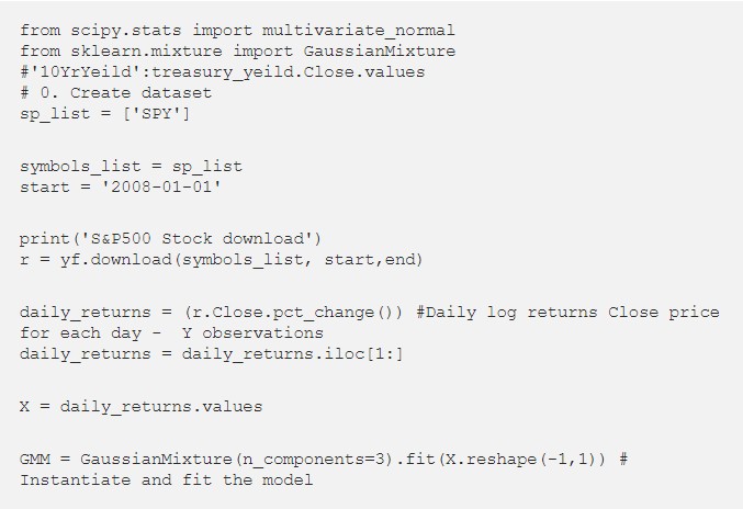
The States for the Gaussian mixture model are found using the Gaussian Mixture model from sklearn and the input data is the daily return for the S&P500.
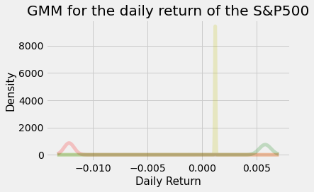
From this above analysis it may also be worth investigating two states.
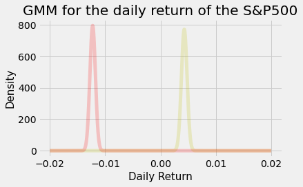
One issue that may arise is convergence. Not in the sense of meeting the criteria of a certain threshold in the EM algorithm, but rather based on the initial conditions, different distributions may take shape depending on the run. Further investigation will be required here.
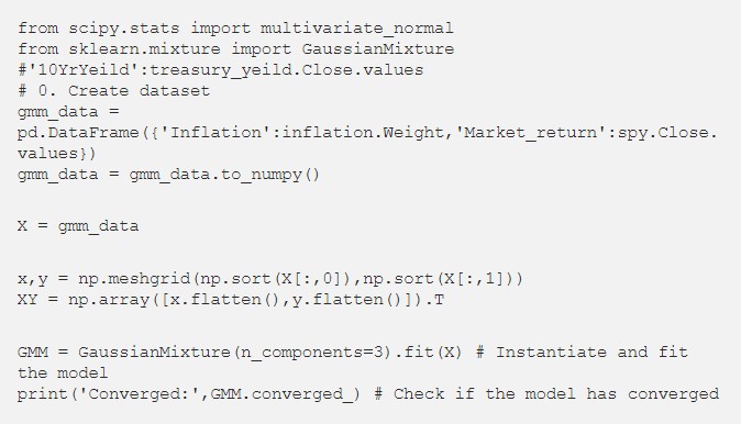
Section 2: Classification of the American economy using Macroeconomics data fit with a GMM
To begin and demonstrate the GMM visually, I will use two-dimensional data or two variables for simplicity. Each corresponding cluster is a multi-normal distribution in three dimensions. In this example, the first dimension is the inflation value (let’s call this X), the second dimension is the S&P500 monthly % return (let’s call this Y) and the third dimension is the joint probability of X&Y. In other words given a certain combination of X and Y what is the probability.
The graph demonstrates one of the main benefits of the GMM over other clustering algorithms. The normal distributions can produce the ellipse shape and this property comes from the covariance matrix.
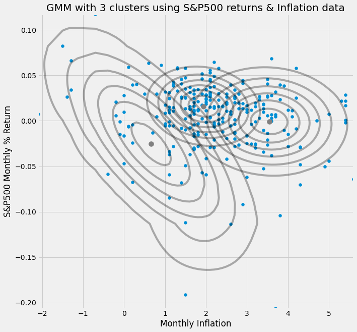
Here the GMM was able to produce three different states given the two dimensional data.
Lastly we can move on to three variables. However, it should be understood that to create a meaningful model, more variables should be considered. In reality, a bevy of different indicators comprise the American economy and its performance.
We can continue and incorporate any number of dimensions, however before you go to n dimensions it is important to understand the correlation structure of the data you are feeding the model. Here, it would make sense to compare to the GDP of the American economy.
Conclusion
This was a simple introduction to how we can apply the GMM to financial markets and the economy. Bear in mind, this was simply an introduction and extensive research is being conducted in this field. The GMM method was introduced to improve the robustness of classifying stock market price data into states.
My recommendation for modelling the market regimes would be to use a GMM and aligning time data to understand the connection between market conditions and the economy
轉貼自Source: medium.datadriveninvestor.com
若喜歡本文,請關注我們的臉書 Please Like our Facebook Page: Big Data In Finance

留下你的回應
以訪客張貼回應