
Summary: Outlining some of the common pitfalls of machine learning for time series forecasting, with a look at time delayed predictions, autocorrelations, stationarity, accuracy metrics, and more.

Time series forecasting is an important area of machine learning. It is important because there are so many prediction problems that involve a time component. However, while the time component adds additional information, it also makes time series problems more difficult to handle compared to many other prediction tasks.
This post will go through the task of time series forecasting using machine learning, and how to avoid some of the common pitfalls.And more specifically, focus on how to evaluate your model accuracy, and show how relying simply on common error metrics such as mean percentage error, R2 score etc. can be very misleading if they are applied without caution.
Example case: Prediction of time series data
The data is split into a training and test set where the first 250 days are used as training data for the model, and we then try to predict the stock index during the last part of the dataset.
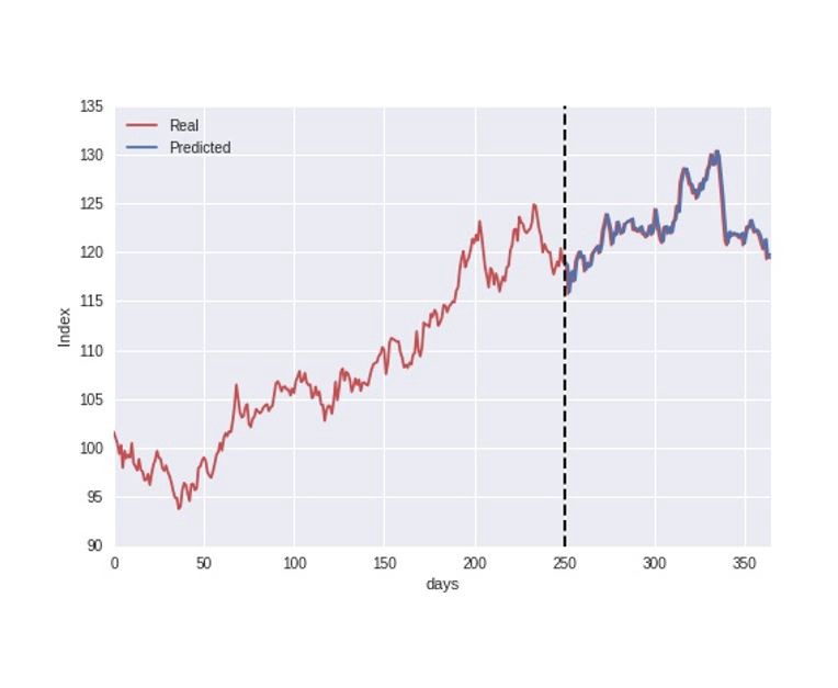
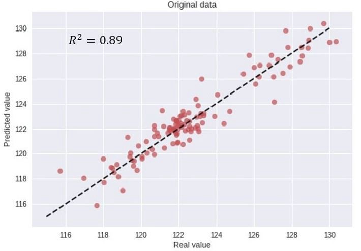
let`s proceed directly to the process of evaluating the model accuracy. Just by visually inspecting the above figure, the model predictions seem to follow the real index closely, indicating a good accuracy. However, to be a bit more precise, we can evaluate the model accuracy by plotting the real vs. predicted values in a scatter plot as illustrated below, and also calculate the common error metric R2 score.
R2 score of 0.89, and seemingly a good match between the real and predicted values.
This is simply WRONG.
The data was actually modeled using a random walk process. As the name indicates, a random walk is a completely stochastic process. Due to this, the idea of using historical data as a training set in order to learn the behavior and predict future outcomes is simply not possible.
Time series data, as the name indicates, differ from other types of data in the sense that the temporal aspect is important. On a positive note, this gives us additional information that can be used when building our machine learning model, that not only the input features contain useful information, but also the changes in input/output over time. However, while the time component adds additional information, it also makes time series problems more difficult to handle compared to many other prediction tasks.
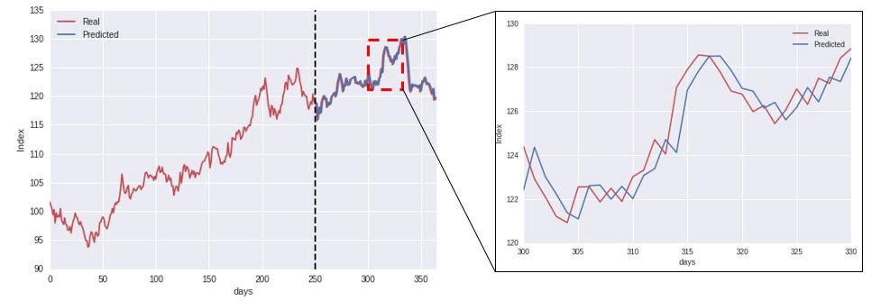
Using an LSTM Network that make predictions according to the data at previous times, we start to see what the model is actually doing.
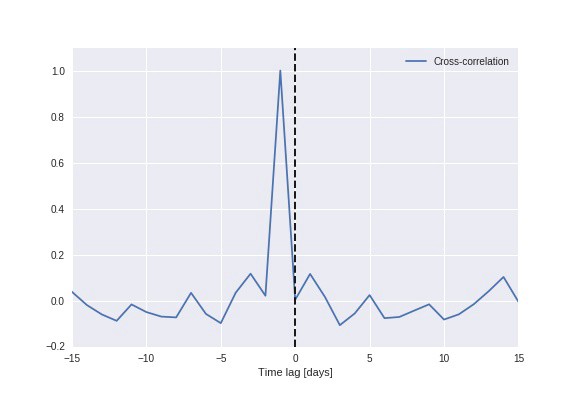
Time series data tend to be correlated in time, and exhibit a significant autocorrelation.Plotting the cross-correlation between the predicted and real value (below figure), we see a clear peak at a time lag of 1 day, indicating that the model simply uses the previous value as the prediction for the future.
Accuracy metrics can be very misleading when used incorrectly
As the example data is generated through a random walk process, the model cannot possibly predict future outcomes. This underlines the important fact that simply evaluating the models predictive powers through directly calculating common error metrics can be very misleading, and one can easily be fooled into being overly confident in the model accuracy.
Stationarity and differencing time series data
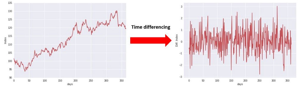
Most statistical forecasting methods are based on the assumption that the time series can be rendered approximately stationary through the use of mathematical transformations. One such basic transformation, is to time-difference the data, as illustrated in the below figure.
Instead of considering the index directly, we are calculating the difference between consecutive time steps.
In that case, it cannot simply use that the data has a strong autocorrelation, and use the value at time “t” as the prediction for “t+1”. Due to this, it provides a better test of the model and if it has learnt anything useful from the training phase, and whether analyzing historical data can actually help the model predict future changes.
Prediction model for time-differenced data
As being able to predict the time-differenced data, let us try this with our model. The results of this test are illustrated in the figure below, showing a scatter-plot of the real vs. predicted values.
This figure indicates that the model is not able to predict future changes based on historical events, which is the expected result in this case, since the data is generated using a completely stochastic random walk process. Being able to predict future outcomes of a stochastic process is by definition not possible, and if someone claims to do this, one should be a bit skeptical…
Click this link for more details: KDnuggets
若喜歡本文,請關注我們的臉書 Please Like our Facebook Page: Big Data In Finance

留下你的回應
以訪客張貼回應