
摘要: A fundamental part of data science
▲Photo by Maxim Hopman on Unsplash
A time series is a sequence of observations or measurements ordered in time. The first picture that comes to mind when talking about time series is usually stock prices. However, time series are ubiquitous.
Yearly rainfall amounts in a geographical location, the daily sales amount of a product in a supermarket, monthly power consumption of a factory, hourly measurements of a chemical process are all examples of time series.
Time series analysis is a fundamental area in data science and has a wide range of applications. If you become an expert in this area, your chance of getting a data scientist job might increase dramatically.
In this article, we will go over 5 must-know terms and concepts in time series analysis.
1. Deterministic and stochastic processes
It is better to start our discussion by distinguishing between deterministic and stochastic processes.
The time-dependent values in a deterministic process can be calculated. For instance, how much you will have in your savings account in two years can be calculated using the initial deposited amount and the interest rate. We can’t really talk about randomness in deterministic processes.
On the other hand, stochastic processes are based on randomness. We cannot calculate the future values in a stochastic process but we can talk about the probability of future values being in a range.
There is a 90% chance that the rainfall amount in California in 2022 will be 21 inches. My assumption is based on the probability distribution of rainfall amounts in California and there is, of course, randomness associated with my assumption.
In this sense, a stochastic process can be considered as a collection of random variables ordered in time. Then, a time series is a realization of a stochastic process.
2. Stationarity
We have just defined time series as a realization of a stochastic process. Stationarity means that the statistical properties of the process that generates the time series do not change over time.
In a stationary time series, we cannot observe a systematic change in mean or variance. Consider we take two intervals from a stationary time series as below:
- N observations from time t to time t + N
- Another N observations from time t + k to t + N + k
The statistical properties of these two intervals are much alike. There is no systematic difference between the mean or variation between these two intervals.
Thus, a stationary time series does not possess
- Seasonality
- Trend
- Periodic fluctuations
The following figure shows a stationary time series. The values might be generated by a random noise but we do not observe a trend or seasonality.

▲(image by author)
The following figure shows a non-stationary time series. We can clearly observe the increasing trend.
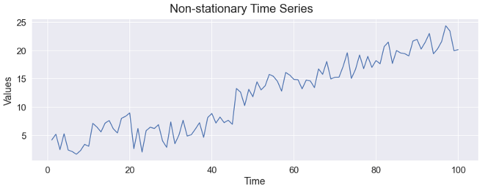
▲(image by author)
3. Autocovariance function
We should first understand what covariance means.
Covariance is a measure of linear dependence between two random variables. It compares two random variables with respect to the deviations from their mean (or expected) value.
The formula of the covariance between random variables X and Y:
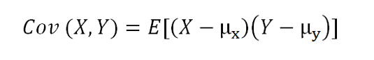
▲Covariance of X and Y
If the values of X and Y change in the same direction (i.e. they both increase or decrease), the covariance between them will be positive.
I tried to explain the covariance and correlation in more detail if you’d like to learn more:
Going back to our discussion on autocovariance, recall that time series is a realization of a stochastic process that can be defined as a sequence of random variables (X₁, X₂, X₃, …).
Assuming we have a stationary time series, let’s take two random variables from this time series:
- Xₜ
- Xₜ ₊ ₖ
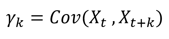
The k is the time difference between these two random variables. The autocovariance function between these two random variables is:
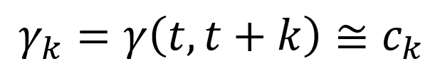
▲Autocovariance function
The autocovariance function only depends on the time difference (i.e. value of k) because we assume stationarity. The properties of a stationary time series do not change when it is shifted in time.
The cₖ is the estimation of the autocovariance function at lag k.
In other words, the properties of the following parts of this time series are the same.
- From Xₜ to Xₜ ₊ ₖ
- From Xₜ ₊ ₙ to Xₜ ₊ ₙ ₊ ₖ
4. Autocovariance coefficients
We now have an understanding of the autocovariance function. The next step is the autocovariance coefficients which are of great importance in time series analysis.
Autocovariance coefficients at different time lags are defined as:
The autocovariance function cannot be computed exactly for a finite time series so we calculate an estimation, cₖ, as follows:
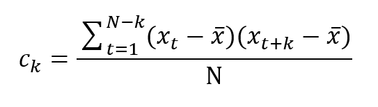
The value x-bar is the sample average.
Consider we want to calculate the autocovariance coefficient for lag 5 of a time series with 50 values (k=5 and N=50).
The numerator of the above equation is calculated for X₁ vs X₆, X₂ vs X₇, …, X₄₀ vs X₄₅. We then take the sum of all the combinations and divide by 50.
We can easily calculate the autocovariance coefficients in R using the acf routine.
Let’s first create a random time series with 50 values.
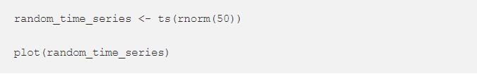
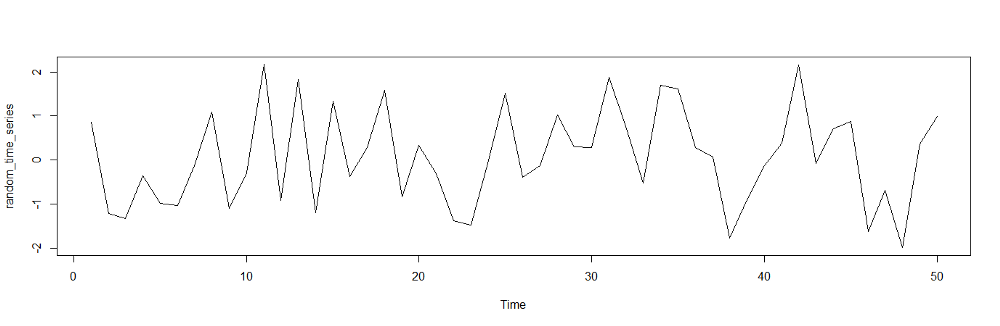
▲Random time series (image by author)
We can calculate the autocovariance coefficients as follows:

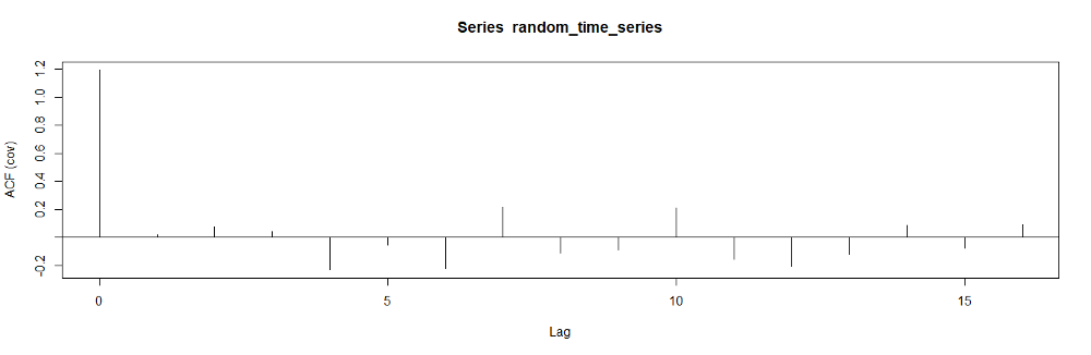
▲Autocovariance coefficients for different time lags (image by author)
5. Autocorrelation function (ACF)
The values of autocovariance coefficients depend on the values in the time series. There is no standard between the autocovariance coefficients of different time series.
What we can use instead is the autocorrelation function (ACF). The autocorrelation coefficient at lag k can be calculated as follows.
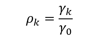
▲Autocorrelation coefficient
We divide the autocovariance coefficient at lag k by the autocovariance coefficient at lag 0.
Similarly, the estimation of the autocorrelation coefficient can be calculated as follows:
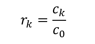
▲The estimation of autocorrelation coefficient
The value of an autocorrelation coefficient is always between -1 and 1.
In R, we can use the acf routine to calculate the autocorrelation coefficients as well.

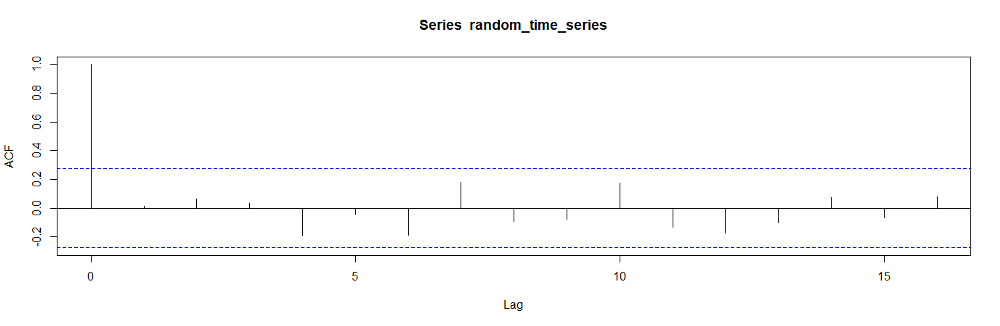
▲ACF plot (image by author)
The autocorrelation coefficients always start with 1 because C₀ / C₀ is equal to 1.
The dashed blue lines represent the significance levels. As we observe in the plot, the correlation values between different time lags are very low because we generated this data randomly.
The ACF plot is also called correlogram.
轉貼自Source: towardsdatascience.com
若喜歡本文,請關注我們的臉書 Please Like our Facebook Page: Big Data In Finance

留下你的回應
以訪客張貼回應