An algorithm to find the best moving average for stock trading

摘要： A simple algorithm for finding the best moving average for every stock or ETF

Moving averages are one of the most used tools in stock trading. Many traders actually use only this tool in their investment toolbox. Let’s see what they are and how we can use Python to fine-tune their features.

What is a moving average?

In a time series, a moving average of period N at a certain time t, is the mean value of the N values before t (included). It’s defined for each time instant excluding the first N ones. In this particular case, we are talking about the Simple Moving Average (SMA) because every point of the average has the same weight. There are types of moving averages that weigh every point in a different way, giving more weight to the most recent data. It’s the case of the Exponential Moving Average (EMA) or the Linear Weighted Moving Average (LWMA).

In trading, the number of previous time series observations the average is calculated from is called period. So, an SMA with period 20 indicates a moving average of the last 20 periods.

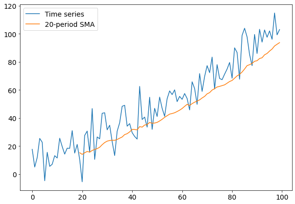
▲A time series with a 20-period Simple Moving Average(來源：towardsdatascience.com)

As you can see, SMA follows the time series and it’s useful to remove noise from the signal, keeping the relevant information about the trend.

Moving averages are often used in time series analysis, for example in ARIMA models and, generally speaking, when we want to compare a time series value to the average value in the past.

How are the moving averages used in stock trading?

Moving averages are often used to detect a trend. It’s very common to assume that if the stock price is above its moving average, it will likely continue rising in an uptrend.

The longer the period of an SMA, the longer the time horizon of the trend it spots.

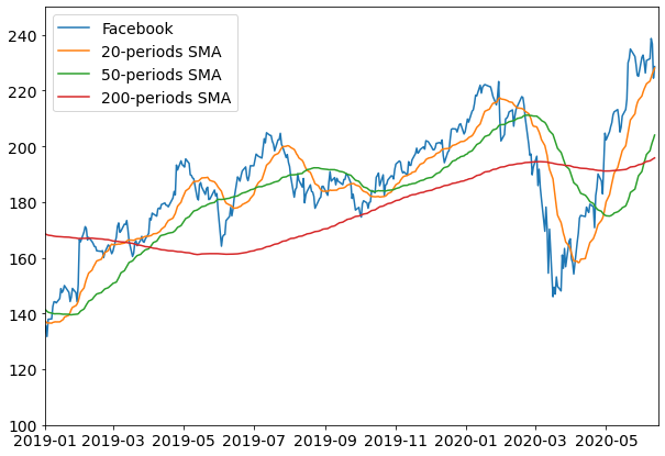
▲Facebook stock price and different SMAs(來源：towardsdatascience.com)

As you can see, short moving averages are useful to catch short-term movements, while the 200-period SMA is able to detect a long-term trend.

Generally speaking, the most used SMA periods in trading are:

• 20 for swing trading
• 50 for medium-term trading
• 200 for long-term trading

It’s a general rule of thumb among traders that if a stock price is above its 200-days moving average, the trend is bullish (i.e. the price rises). So they are often looking for stocks whose price is above the 200-periods SMA.

How can I choose the SMA period?

In order to find the best period of an SMA, we first need to know how long we are going to keep the stock in our portfolio. If we are swing traders, we may want to keep it for 5–10 business days. If we are position traders, maybe we must raise this threshold to 40–60 days. If we are portfolio traders and use moving averages as a technical filter in our stock screening plan, maybe we can focus on 200–300 days.

Choosing the investment period is a discretionary choice of the trader. Once we have determined it, we must try to set a suitable SMA period. We have seen 20, 50 and 200 periods, but are they always good? Well not really.

Markets change a lot during the time and they often make traders fine-tune their indicators and moving averages in order to follow volatility burst, black swans and so on. So there isn’t the right choice for the moving average period, but we can build a model that self-adapts to market changes and auto-adjust itself in order to find the best moving average period.

The algorithm for the best moving average

The algorithm I propose here is an attempt to find the best moving average according to the investment period we choose. After we choose this period, we’ll try different moving averages length and find the one that maximizes the expected return of our investment (i.e. if we buy at 100 and after the chosen period the price rises to 105, we have a 5% return).

The reason of using the average return after N days as an objective function is pretty simple: we want our moving average to give us the best prediction of the trend according to the time we want to keep stocks in our portfolio, so we want to maximize the average return of our investment in such a time.

In practice, we’ll do the following:

• Take some years of daily data of our stock (e.g. 10 years)
• Split this dataset into training and test sets
• Apply different moving averages on the training set and, for each one, calculate the average return value after N days when the close price is over the moving average (we don’t consider short positions for this example)
• Choose the moving average length that maximizes such average return
• Use this moving average to calculate the average return on the test set
• Verify that the average return on the test set is statistically similar to the average return achieved on the training set

The last point is the most important one because it performs cross-validation that helps us avoid overfitting after the optimization phase. If this check is satisfied, we can use the moving average length we found.

For this example, we’ll use different stocks and investment length. The statistical significance of the mean values will be done using Welch’s test.

An example in Python

Short-term investment

First of all, we must install yfinance library. It’s very useful for downloading stock data.

Then we can import some useful packages:

Let’s assume we want to keep the SPY ETF on S&P 500 index for 2 days and that we want to analyze 10 years of data.

Now we can download our data and calculate the return after 2 days.

Now we can perform the optimization for searching the best moving average. We’ll do a for loop that spans among 20-period moving average and 500-period moving average. For each period we split our dataset in training and test sets, then we’ll look only ad those days when the close price is above the SMA and calculate the forward return. Finally, we’ll calculate the average forward return in training and test sets, comparing them using a Welch’s test.

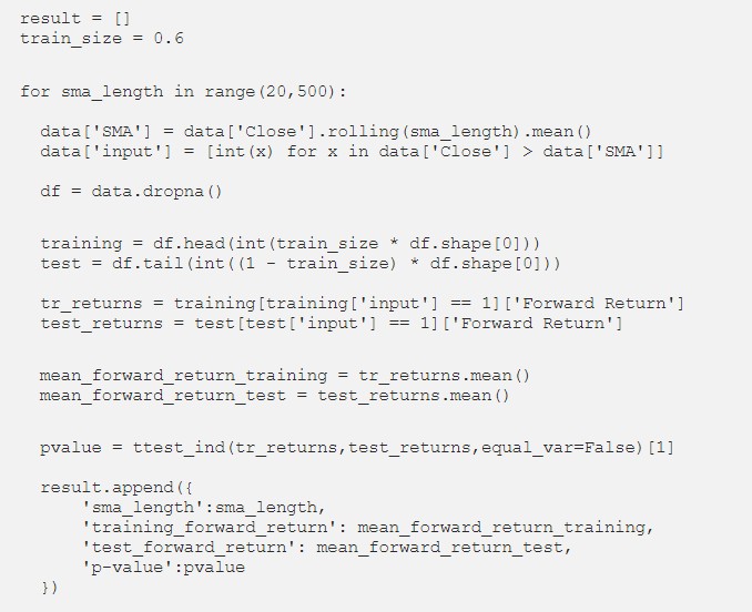
We’ll sort all the results by training average future returns in order to get the optimal moving average.

The first item, which has the best score, is:

As you can see, the p-value is higher than 5%, so we can assume that the average return in the test set is comparable with the average return in the training set, so we haven’t suffered overfitting.

Let’s see the price chart according to the best moving average we’ve found (which is the 479-period moving average).

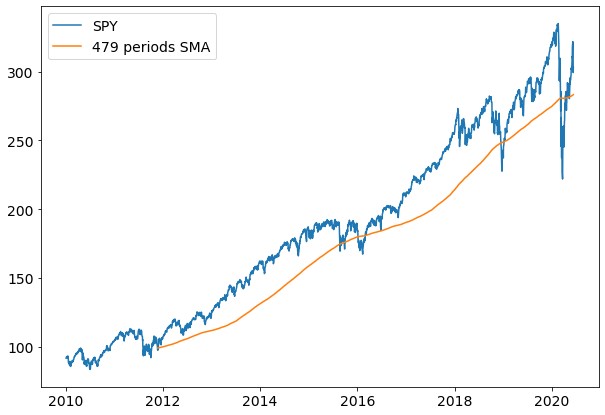
▲圖片來源：towardsdatascience.com

It’s clear that the price is very often above the SMA.

Long-term investment

Now, let’s see what happens if we set n_forward = 40 (that is, we keep our position opened for 40 days).

The best moving average produces these results:

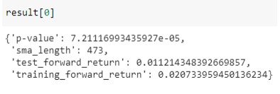
As you can see, the p-value is lower than 5%, so we can assume that the training phase has introduced some kind of overfitting, so we can’t use this SMA in the real world. Another reason could be that volatility has changed too much and the market needs to stabilize before making us invest in it.

Finally, let’s see what happens with a Gold-based ETF (ticker: GLD) with 40-days investment.

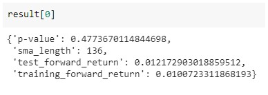
p-value is quite high, so there’s no overfitting.

The best moving average period is 136, as we can see in the chart below.

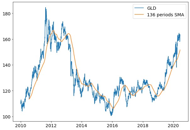
▲圖片來源：towardsdatascience.com

Conclusions

In this article, we’ve seen a simple algorithm to find the best Simple Moving Average for stock and ETF trading. It can be easily applied every trading day in order to find, day by day, the best moving average. In this way, a trader can easily adapt to market changes and to volatility fluctuations.

詳文見 ： towardsdatascience.com

若喜歡本文，請關注我們的臉書 Please Like our Facebook Page： 　　　Big Data In Finance